本文介绍如何使用 ARIMA 预测 COVID-19 趋势。数据来源为 CSSEGISandData/COVID-19

选择参数

传统的做法是利用差分观察数据是否稳定来确定 d,利用 自相关图 ACF 和 偏自相关图 PACF 分别确定 q,p 的值。下面尝试一种用网格搜索法来确定参数的思路。

对于每日新增确诊病例数,大致确定 (p, d, q),以及 seasonal-(P, D, Q) 的范围,时序周期为 7 天,通过迭代不同参数的组合来获取最佳参数。在评估和比较不同参数的模型时,使用 AIC 值来评估,AIC 的值越小,则模型越优。

 1
 2
 3
 4
 5
 6
 7
 8
 9
10
11
12
13
14
15
16
17
18
19
20
21
22
23
24
25
26
27
28
29
30
31
32
33
34
35
36
37
38
39
40
41
42
43
44
import itertools, warnings
import matplotlib.pyplot as plt
import pandas as pd

from statsmodels.tsa.arima.model import ARIMA

# 读取网页,提取数据
df = pd.read_csv('https://raw.githubusercontent.com/CSSEGISandData/COVID-19/master/csse_covid_19_data/csse_covid_19_time_series/time_series_covid19_confirmed_global.csv')
df = df.iloc[:, 4:]                               # 从第4列开始读取,弃掉经纬度等信息
df.loc['Worldwide'] = df.apply(lambda x: x.sum()) # 新增一行全球累计数据,并按列求和
df = df.iloc[-1:, :].T                            # 提取最后一行,全部列,即全球累计这一行,并转置行列
df.index = pd.DatetimeIndex(df.index)             # 将索引转换为时间序列
df = df.diff().dropna()                           # 计算一阶差分,获得每日新增数量

# 确定模型参数
p = range(0, 5)                                   # autoregressive (AR) order
d = range(0, 2)                                   # differencing order
q = range(0, 2)                                   # moving average (MA) order
pdq = list(itertools.product(p, d, q))

P = range(0, 8)                                   # seasonal AR order
D = range(0, 2)                                   # seasonal differencing order
Q = range(0, 2)                                   # seasonal MA order
seasonal_pdq = [(x[0], x[1], x[2], 7)
                for x in list(itertools.product(P, D, Q))]

warnings.filterwarnings('ignore')
aic_dict = {}
for param in pdq:
    for param_seasonal in seasonal_pdq:
        try:
            model = ARIMA(df,
                          order=param,
                          seasonal_order=param_seasonal,
                          enforce_stationarity=False,
                          enforce_invertibility=False)
            results = model.fit()
            aic_dict.update({results.aic: [param, param_seasonal]})
            print('ARIMA{}x{} - AIC:{}'.format(param, param_seasonal, results.aic))
        except:
            continue

# 找出最小值
print('矩阵最小组合为:', aic_dict[min(aic_dict.keys())])
 1
 2
 3
 4
 5
 6
 7
 8
 9
10
11
12
13
14
ARIMA(0, 0, 0)x(0, 0, 0, 7) - AIC:6661.80851161719
ARIMA(0, 0, 0)x(0, 0, 1, 7) - AIC:5356.970830120317
ARIMA(0, 0, 0)x(0, 1, 0, 7) - AIC:4747.066788868986
ARIMA(0, 0, 0)x(0, 1, 1, 7) - AIC:4580.640379744944
ARIMA(0, 0, 0)x(1, 0, 0, 7) - AIC:4772.019450121369
ARIMA(0, 0, 0)x(1, 0, 1, 7) - AIC:4744.755708646536
ARIMA(0, 0, 0)x(1, 1, 0, 7) - AIC:4585.865237068969
ARIMA(0, 0, 0)x(1, 1, 1, 7) - AIC:4546.8779891241575
ARIMA(0, 0, 0)x(2, 0, 0, 7) - AIC:4589.485136017654
ARIMA(0, 0, 0)x(2, 0, 1, 7) - AIC:4581.982143665322
...
...
...
矩阵最小组合为: [(6, 1, 0), (7, 1, 0, 7)]

检验模型

通过“网格搜索”找到了最佳拟合模型的参数,使用最佳参数值建立一个新的 ARIMA 模型。
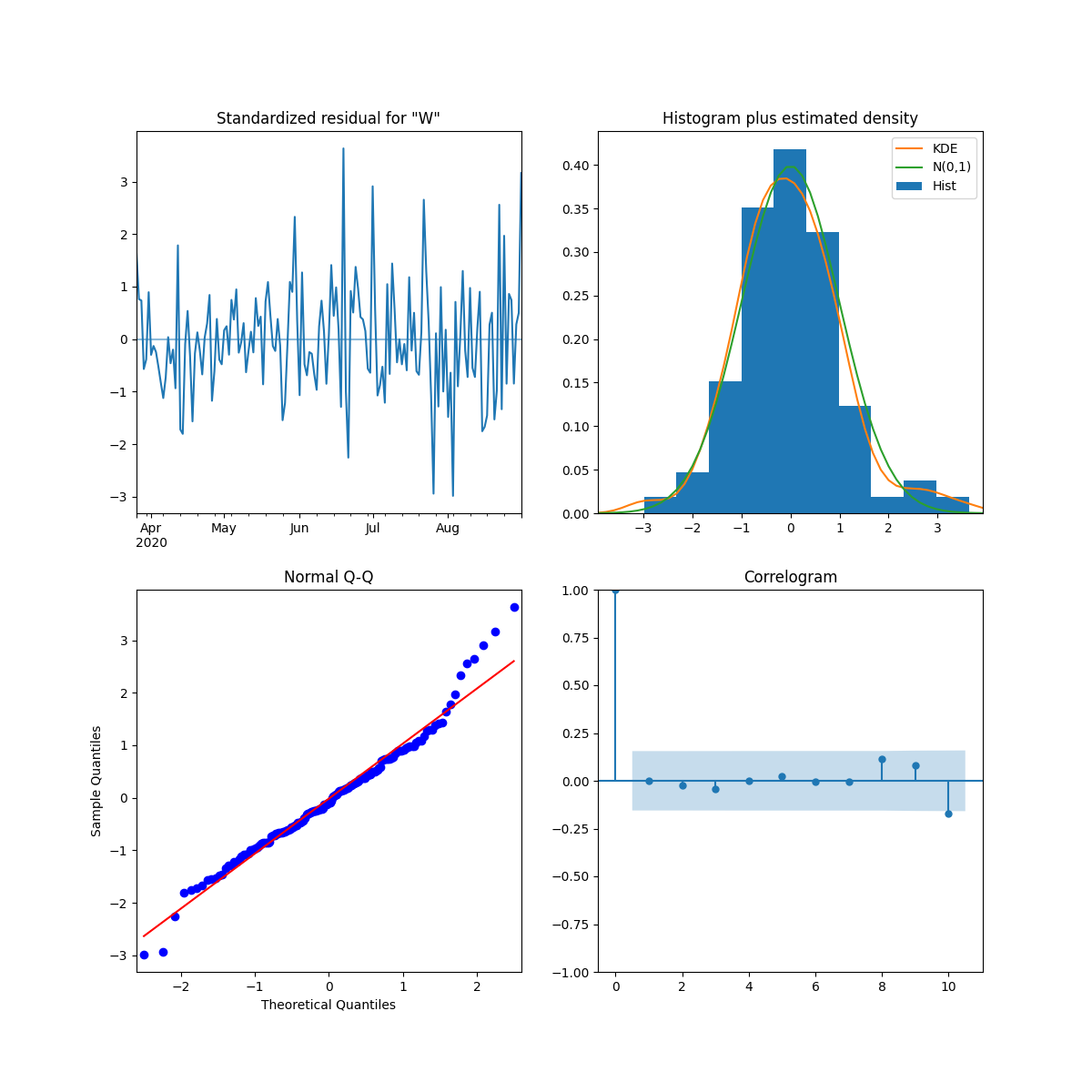
 1
 2
 3
 4
 5
 6
 7
 8
 9
10
11
12
13
14
15
16
17
18
19
20
21
22
# 建立模型
model = ARIMA(df,
              order=(6, 1, 0),
              seasonal_order=(7, 1, 0, 7),
              enforce_stationarity=False,
              enforce_invertibility=False)
results = model.fit()

# 计算相关度参数表
print(results.summary())

# 绘制诊断图
results.plot_diagnostics(figsize=(12, 12))
plt.savefig('images/diagnostics.png')

# 校验对比数据
df['Validating'] = results.predict(start='2020-02-01',
                                   dynamic=False)

ax = df.plot(figsize=(12, 8))
ax.set_xlabel('')
plt.savefig('images/validation.png', bbox_inches='tight')
 1
 2
 3
 4
 5
 6
 7
 8
 9
10
11
12
13
14
15
16
17
18
19
20
21
22
23
24
25
26
27
28
29
30
31
32
                                    SARIMAX Results
=======================================================================================
Dep. Variable:                       Worldwide   No. Observations:                  222
Model:             ARIMA(6, 1, 0)x(7, 1, 0, 7)   Log Likelihood               -1695.973
Date:                         Sun, 06 Sep 2020   AIC                           3419.945
Time:                                 20:04:03   BIC                           3462.910
Sample:                             01-23-2020   HQIC                          3437.393
                                  - 08-31-2020
Covariance Type:                           opg
==============================================================================
                 coef    std err          z      P>|z|      [0.025      0.975]
------------------------------------------------------------------------------
ar.L1         -0.6802      0.079     -8.583      0.000      -0.836      -0.525
ar.L2         -0.4023      0.099     -4.058      0.000      -0.597      -0.208
ar.L3         -0.3618      0.114     -3.170      0.002      -0.586      -0.138
ar.L4         -0.1344      0.103     -1.303      0.192      -0.337       0.068
ar.L5         -0.0971      0.102     -0.954      0.340      -0.297       0.102
ar.L6          0.1115      0.106      1.049      0.294      -0.097       0.320
ar.S.L7       -0.4496      0.103     -4.373      0.000      -0.651      -0.248
ar.S.L14      -0.3734      0.108     -3.467      0.001      -0.584      -0.162
ar.S.L21      -0.0713      0.093     -0.767      0.443      -0.253       0.111
ar.S.L28      -0.2144      0.099     -2.170      0.030      -0.408      -0.021
ar.S.L35       0.0025      0.120      0.021      0.983      -0.233       0.238
ar.S.L42      -0.1020      0.125     -0.817      0.414      -0.347       0.143
ar.S.L49      -0.1413      0.110     -1.281      0.200      -0.357       0.075
sigma2      9.749e+07   5.55e-10   1.76e+17      0.000    9.75e+07    9.75e+07
===================================================================================
Ljung-Box (L1) (Q):                   0.00   Jarque-Bera (JB):                15.44
Prob(Q):                              0.99   Prob(JB):                         0.00
Heteroskedasticity (H):               2.77   Skew:                             0.43
Prob(H) (two-sided):                  0.00   Kurtosis:                         4.26
===================================================================================

如上图:

  • 左上观察残差的均值是否接近 0;
  • 右上看残差是否接近正态分布;
  • 左下 Q-Q 图查看是否接近红线;
  • 右下查看相关性是否在阈值之内。

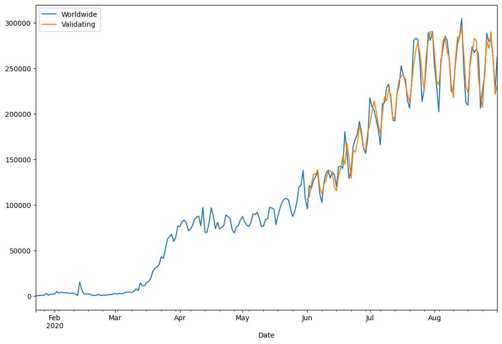
如上图,预测的红线与实际的蓝线非常接近。

预测结果

 1
 2
 3
 4
 5
 6
 7
 8
 9
10
11
12
13
14
15
16
17
# 预测 30 天数据
pred = results.get_forecast(steps=30)

# 图表呈现
ax = df.plot(figsize=(12, 8))
pred.predicted_mean.plot(ax=ax, label='Forecasting')
pred_ci = pred.conf_int()
ax.fill_between(pred_ci.index,
                pred_ci.iloc[:, 0],
                pred_ci.iloc[:, 1],
                color='k',
                alpha=.25)
ax.set_xlabel('')
plt.legend()
plt.savefig('images/covid.png', bbox_inches='tight')

return 'images/covid.png'

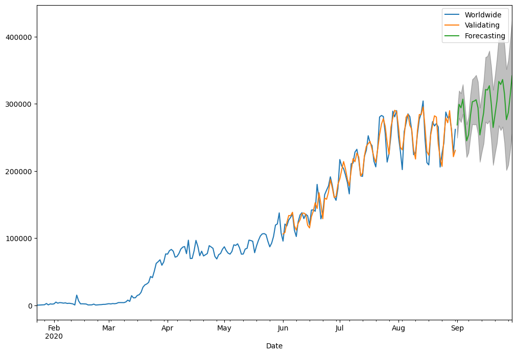
上图就是每日新增确诊病例在接下来 30 天的走势。

用同样的方法,调整不同的参数,还可以预测累计确诊病例下个月的走势。
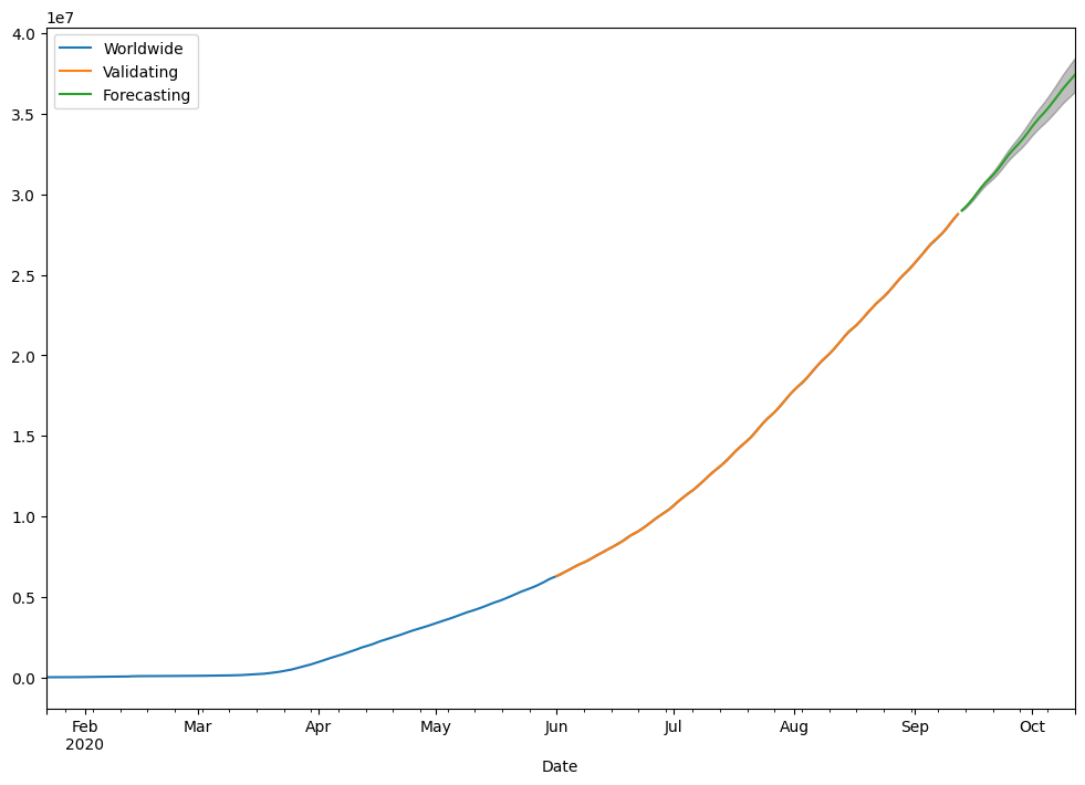
 挑两天的预测值如下表, 到时做个对比, 已更新:

日期预测值下限预测值上限预测值均值实际值
2020/10/0133643630347416503419264034290251
2020/10/1035913420378049603685919037207057